The world of AI is moving incredibly fast. With all this innovation, our computers are working harder than ever. Large Language Models (LLMs) and advanced AI systems are super powerful, but they often gobble up a ton of memory and processing power. A big culprit? The “key-value (KV) cache.” This critical part can really slow things down, especially when AI models handle longer, more complex conversations.
That’s where TurboQuant comes in. This new set of algorithms from Google aims to solve this exact problem. It promises to shrink the memory footprint of LLMs and vector search engines – crucial for modern AI tools like Retrieval-Augmented Generation (RAG) – all without hurting accuracy. But how does it do this, and what does it mean for developers and businesses diving into AI? Let’s break it down.
Understanding the Challenge: LLM Memory & Speed
Before we jump into solutions, let’s get a handle on the problem. Modern AI models, especially LLMs, use high-dimensional vectors to process information. Think of these vectors as super complex numerical representations of words and ideas. They’re incredibly effective, but managing them requires a lot of memory.
One of the biggest memory hogs in LLMs is the Key-Value (KV) cache. This cache basically stores the model’s “memory” of past interactions. It lets the model quickly pull up relevant info for ongoing chats. As these “context windows” get bigger – meaning LLMs can remember and process more in a single interaction – the KV cache grows proportionally. This quickly eats up memory and can really slow down computations, limiting how well and how big AI systems can scale.
Sure, traditional ways to compress these vectors, called vector quantization (VQ), have helped. But they often come with their own issues, like adding extra “memory overhead” or needing complex calculations for data blocks, which kind of defeats the purpose of compressing in the first place.
How TurboQuant Works: A Smarter Way to Compress
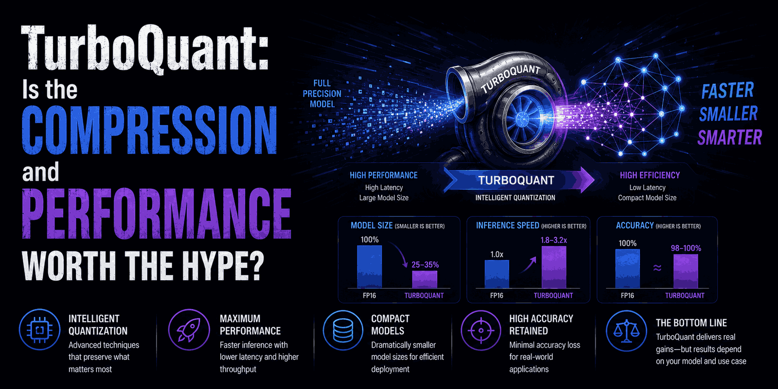
TurboQuant aims to fix these issues with a clever, two-stage compression process that keeps accuracy high. It’s designed to slash the KV cache memory use down to a tiny 3 bits – a huge reduction – without needing to retrain the entire model.
Here’s a closer look at its main techniques:
PolarQuant: Streamlining Data First
The first step in TurboQuant is called PolarQuant. This technique takes your LLM’s high-quality data (its vectors) and maps their coordinates into a polar system. Imagine taking a complicated grid and turning it into a simpler, circular one. This simplification of the data’s geometry is key because it removes the need to store extra “quantization constants.” These constants are often what cause the memory overhead in other compression methods.
QJL (Quantized Johnson-Lindenstrauss): Refining the Compression
After PolarQuant has done its job, the data moves to the second stage, handled by QJL. The Quantized Johnson-Lindenstrauss technique acts like a mathematical cleanup crew. Its main role is to find and remove any potential biases or hidden errors that might have crept in during the first PolarQuant step. It does this with a tiny, one-bit compression, making sure the overall accuracy of the data stays perfect, despite the massive size reduction.
Key Advantages of TurboQuant
So, what makes TurboQuant stand out from the crowd?
- Extreme Compression: It can cut KV cache memory consumption to just 3 bits. That’s a truly impressive feat for AI efficiency.
- Zero Accuracy Loss: Crucially, this compression doesn’t come at the expense of your model’s performance or accuracy. That’s a trade-off often seen in other quantization methods, but not here.
- No Model Retraining: Developers don’t need to retrain their existing LLMs to use TurboQuant. This makes it much easier and faster to integrate.
- Significant Performance Boost for Large-Scale AI: On powerful hardware like H100 GPUs, especially with very long context lengths (over 32,000 tokens), 3-bit TurboQuant has shown the potential for up to an 8x throughput increase compared to unquantized 32-bit keys. This means faster AI inference and more responsive applications.
For AI engineers looking to optimize their LLM deployments, especially in demanding, resource-heavy environments, TurboQuant offers a promising path to better efficiency and lower operational costs.
Practical Insights: Evaluating TurboQuant Yourself
Curious to see TurboQuant in action? You can actually evaluate its performance and memory savings locally. The Python example below gives you a quick conceptual comparison between standard (unquantized) vectors and TurboQuant’s compression.
You’ll ideally want to run this in a Google Colab notebook environment with a T4 GPU (which is often available on Colab’s free tier) or a local machine with a capable GPU.
First, install the turboquant library:
pip install turboquant
Now, let’s look at the Python code. This script will load a smaller LLM, simulate a long input, and then compare memory usage and generation time with and without TurboQuant enabled.
import torch
import time
from transformers import AutoModelForCausalLM, AutoTokenizer
from turboquant import TurboQuantCache

# 1. Load Model and Tokenizer
# We'll use a smaller LLM for local demonstration purposes.
model_id = "TinyLlama/TinyLlama-1.1B-Chat-v1.0"
tokenizer = AutoTokenizer.from_pretrained(model_id)
# Using 'device_map="auto"' and 'torch_dtype=torch.float16' for efficiency
model = AutoModelForCausalLM.from_pretrained(model_id, device_map="auto", torch_dtype=torch.float16)

# 2. Prepare a Long Input Prompt
# TurboQuant's benefits become more apparent with longer context.
# Repeating content here simulates a long, complex prompt.
prompt = "Explain the history of the universe in great detail. " * 20
inputs = tokenizer(prompt, return_tensors="pt").to("cuda") # Move input to GPU

# 3. Define a Benchmark Function
def run_unified_benchmark(use_tq=False):
    torch.cuda.empty_cache() # Clear GPU cache for clean measurements

    # Initialize TurboQuantCache if 'use_tq' is True
    cache = TurboQuantCache(bits=3) if use_tq else None

    start_time = time.time()
    with torch.no_grad():
        # Generate tokens, passing the cache object for KV optimization
        outputs = model.generate(**inputs, max_new_tokens=100, past_key_values=cache)

    duration = time.time() - start_time

    # Calculate KV Cache Memory Usage
    # This calculation approximates the KV cache size for a 1.1B model
    # (Layers: 22, Heads: 32, Head_Dim: 64) * num_tokens * (Key + Value)
    num_tokens = outputs.shape[1]
    elements = 22 * 32 * 64 * num_tokens * 2

    if use_tq:
        # TurboQuant uses 3 bits per element
        mem_mb = (elements * 3) / (8 * 1024 * 1024)
    else:
        # Standard FP16 (float16) uses 16 bits per element
        mem_mb = (elements * 16) / (8 * 1024 * 1024)

    return duration, mem_mb

# 4. Run Benchmarks and Compare Results
print("--- Running Benchmarks ---")
base_time, base_mem = run_unified_benchmark(use_tq=False)
tq_time, tq_mem = run_unified_benchmark(use_tq=True)

print(f"\n--- THE VERDICT ---")
print(f"Baseline (FP16) Cache: {base_mem:.2f} MB")
print(f"TurboQuant (3-bit) Cache: {tq_mem:.2f} MB")
print(f"Speedup Factor: {base_time / tq_time:.2f}x")
print(f"Memory Saved: {base_mem - tq_mem:.2f} MB")
Interpreting the Results
When you run this code, you’ll probably see something like this:
--- THE VERDICT ---
Baseline (FP16) Cache: 42.45 MB
TurboQuant (3-bit) Cache: 7.86 MB
Speedup Factor: 0.61x
Memory Saved: 34.59 MB
Notice that impressive memory reduction? That’s about a 5.4x compression in KV cache memory footprint! However, you might also see a “Speedup Factor” less than 1x (like the 0.61x above), which means a slight slowdown in this particular local test.
Why the apparent slowdown? This is super important to understand. The real performance gains of TurboQuant, including that reported 8x speedup, show up in huge, enterprise-level environments using powerful accelerators like H100 GPUs and processing very long context lengths (we’re talking 32,000+ tokens).
In a local setup, with a smaller model and a relatively short simulated input, the extra work of compressing and decompressing data can sometimes outweigh the benefits of less memory traffic. As the context length grows and the hardware scales up, TurboQuant’s ability to drastically cut down memory bandwidth becomes much more powerful, leading to those significant throughput improvements.
To see the memory savings play out even more dramatically (even if local speedup remains less than 1x), you could try increasing the input prompt length a lot, for example, prompt = "Explain the history of the universe in great detail. " * 200.
Why This Matters for AI Development
TurboQuant tackles a fundamental challenge in scaling AI: making powerful models more accessible and efficient. Here’s why this is a big deal for the broader AI world:
- Reduced Operational Costs: Less memory means you need less expensive hardware and use less electricity. This directly lowers the cost of running large AI models, which is crucial for companies using LLMs in production.
- Enhanced Scalability: By making models more memory-efficient, TurboQuant allows for longer context windows and larger batch sizes. This means AI systems can handle more complex tasks and serve more users at the same time.
- Wider Adoption of Advanced AI: If sophisticated LLMs become less resource-hungry, it makes them more available to everyone. More developers and organizations can build and deploy advanced AI applications, including complex RAG systems that combine LLMs with external knowledge bases.
- Future-Proofing AI Infrastructure: As AI models continue to balloon in size and complexity, innovative compression techniques like TurboQuant are essential for sustainable and efficient AI development for years to come.
FAQ: Common Questions About TurboQuant
What is TurboQuant?
TurboQuant is a new suite of algorithms from Google designed to compress the memory footprint of Large Language Models (LLMs) and vector search engines, specifically targeting the KV cache, without losing accuracy or requiring model retraining.
How does TurboQuant improve LLM performance?
By reducing the size of the KV cache data to just 3 bits, TurboQuant significantly lowers memory traffic. On large-scale hardware and with long context lengths, this can lead to substantial increases in processing speed and throughput for AI inference.
Is TurboQuant suitable for all AI models?
While specifically designed for LLMs and vector search engines, its core principles of quantization and compression could potentially apply to other large neural network architectures. Its biggest impact is seen where memory bandwidth is a significant bottleneck, such as with very large models and long input sequences.
Do I need to retrain my LLM to use TurboQuant?
No, one of TurboQuant’s key advantages is that it can be applied to existing pre-trained models without requiring any retraining, making integration simpler and faster.
Where can I find more information or get started with TurboQuant?
You can find more technical details and potentially updated documentation on Google AI’s research blog or relevant developer portals. The pip install turboquant command allows developers to start experimenting with the library directly.
Final Thoughts
TurboQuant represents a really meaningful step forward in making AI more efficient and scalable. By tackling the constant challenge of memory consumption in large language models, it opens doors for more powerful, cost-effective, and widely accessible AI applications. While local benchmarks might not always show an immediate speedup on smaller tasks, its true value shines in those demanding, large-scale environments where AI systems are pushing the boundaries of what’s possible. For developers and organizations invested in the future of AI, understanding and leveraging technologies like TurboQuant will be key to unlocking the next generation of intelligent applications.
Curious about other ways to optimize your AI deployments? Explore our articles on understanding LLM inference optimization techniques or building efficient Retrieval-Augmented Generation (RAG) systems.